BIBoP 1 - Intro and Machine Learning :: Jakub Duchniewicz

Introduction

Hi! My name is Jakub Duchniewicz and welcome to Brother Industry Band of Power.

In this post series we plan to describe our progress with the BIBoP project and shed some light on various issues we had to tackle along the way.

Be sure to check the [official repository] of this project!

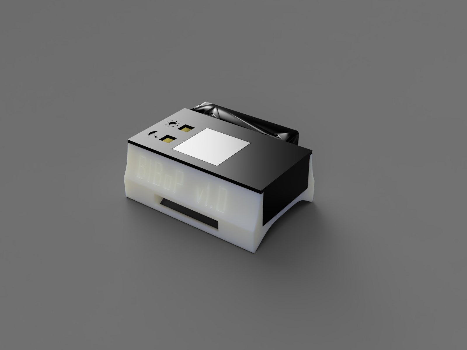
Here is a small sneak-peek of how the device will look like once assembled:

Why?

Since I haven’t posted in a while, a small update on the reasons behind this blog post series and why ultimately my last project ([Envidrawer]) was not documented here.

The reason is quite obvious: I am already documenting the project on the [official contest website] and I am bringing here the best nitbits from there.

Also, this project touches on so many domains and digs into several obscure areas (SAMD21 MCU programming, BP estimation from PPG, AWS Lambda over TLS/SSL…), it would be a shame not to document them!

Envidrawer

As for the [Envidrawer] project, I finished it in quite busy time of my life (changing countries, being sick) so I did not move it to this website. Maybe one day…

Nevertheless, be sure to check [some] [cool] [concepts] we came up with during development of the Envidrawer project.

Project overview

Similarly as with Envidrawer, I teamed up with Michał and Szymon to create a solution to an important problem which the humanity is currently facing or will be facing in near future. Unfortunately, the project is during their exam time on universities and it is mostly my responsibility 😄 (not that I am complaining!).

Our project is a wearable band which that will measure oxygen saturation, pulse, and body temperature of the potential patient. It will automatically connect to Wi-Fi and on reaching certain thresholds call in the emergency team for hospitalization. Being a cheap and easy to manufacture device, it could be distributed to the patients from high-risk groups which upon falling sick could make use of it. The true beauty lies in the fact that it could stay after the pandemic, once again moving healthcare closer to its recipients.

In other words, we want to provide people with affordable, easy-to-use smart-bands which will measure their vital signals and report any abnormalities to medical staff and to the users themselves.

In the picture below you can see the high-level overview of the project (the real photos will come in as soon as the 3D printed case is ready!).

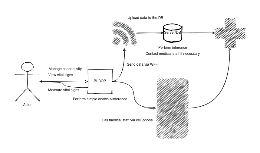
Every project has to be powered by [Arduino Nano 33 IoT], thus I decided to make use of some ready made Arduino libraries, such as WiFiNINA or BearSSL which are necessary for secure wireless communication. At the moment of writing this post I am waist-deep in the SAMD21 datasheet and trying to enable external interrupts in low power modes, since Arduino development framework does not provide all conceivable solutions.

Because of shortages in the developer team, the project may not achieve all of its goals on-time, but it definitely is worth spending some time on after the contest ends. After all, having your own smart-band is quite exciting 😁.

I - First steps

Setting up the development environment is one of the first steps every developer has to undertake, so that is what I also had to do. The SAMD boards require their own Board Support Package which is best downloaded using the official Arduino IDE.

First of all we need to setup our build and editing environment.

Enter Makefiles.

DISCLAIMER - This is fairly technical paragraph so feel free to scroll down for the Machine Learning related content

Why use Makefiles, when we have Arduino IDE?

We have Arduino IDE, right. But apart from providing users with handy building scripts and libraries + toolchains management, it failed to meet the IDE standards in term of code editing. Since I am heavy vim user, I wanted to write my code in familiar environment and with handy shortcuts and handy tools.

This is just one reason behind it, the other being code extensibility, compiler choice and language version freedom. Assuming you want to have your own libraries as a part of a bigger project, Arduino IDE does not present you with an easy way to do it - with a custom Makefile you can structure your project as desired. This unfortunately is by no means out of the box solution, but I was able to polish some rough edges and possibly make it easier to fall in step for whoever reads this post.

Cloning and setting up

Assuming you have read this far and are willing to create your own Makefile-based Arduino project, you need to create the folder structure or simply fork/clone this project. You have a bunch of unnecessary files to delete, such as exemplary Makefiles and mock libraries. Instead what you need to do is follow the INSTALL.md which guides you by hand mostly.

Once you have the Makefile in the project directory (src/ProjectName/Makefile), you have to fill it with some necessary variables which are used during the process of building the binary and during the flashing and debugging the code. Exemplary Makefile can be found below:

# For now makefile will be in this file, we will change it later
PROJECT_DIR       = $(shell dirname $(shell dirname $(shell pwd)))

ARDMK_DIR         = $(PROJECT_DIR)/Arduino-Makefile
ARDUINO_PACKAGE_DIR = $(HOME)/.arduino15/packages
ARDUINO_DIR       = /usr/share/arduino
USER_LIB_PATH     :=  $(realpath $(PROJECT_DIR)/lib)
BOARD_TAG         = nano_33_iot
MONITOR_PORT      = /dev/ttyACM*
MONITOR_BAUDRATE  = 115200
AVR_TOOLS_DIR     = /usr
AVRDUDE           = /usr/bin/avrdude
CFLAGS_STD        = -std=gnu11
CXXFLAGS_STD      = -std=gnu++17
CXXFLAGS         += -pedantic -Wall -Wextra
LDFLAGS          += -fdiagnostics-color

### OBJDIR
### Don't touch this!
### This is were you put the binaries you just compile using 'make'
CURRENT_DIR       = $(shell basename $(CURDIR))
OBJDIR            = $(PROJECT_DIR)/build/$(CURRENT_DIR)/$(BOARD_TAG)

include $(ARDMK_DIR)/Sam.mk

As you can see, not much is needed to make all of this work (most of the variables are pre-filled and just have to be tweaked by you - hopefully you won’t need to know the Makefile content by heart like I did while repairing it ). Remember to point the USER_LIB_PATH to the ProjectRoot/lib path and to symlink/copy the libraries you plan to use to this directory.

The GitHub repository README mentions that you have to set the BOARD_TAG and BOARD_SUB if you have boards which have these two parameters, but for the Arduino Nano 33 IoT we just need to set the BOARD_TAG to nano_33_iot

Lastly, because the original Makefiles are for the regular AVR Arduinos, you need to change the last line which includes the main Makefile from include $(ARDMK_DIR)/Arduino.mk to include $(ARDMK_DIR)/Sam.mk

Polishing the rough edges

If you tried compiling right now, you would be met by some errors about missing LTO plugins during running the binary linking step. The reason for this was fixed upstream but is not ported to the Makefile you have in the project, so I suggest changing the git submodule to the upstream. You can do it with following commands:

git submodule deinit Arduino-Makefile
git rm Arduino-Makefile
# now add the gitmodule
git submodule add https://github.com/sudar/Arduino-Makefile Arduino-Makefile
git submodule update --init --recursive

The --recursive flag was needed in case the submodule includes other submodules.

Having the upstream Makefile, we have some problems fixed. Unfortunately this does not fix the libraries you create by yourself so I just add the LTO plugin by myself by adding the following line to the Arduino.mk:

# SPECIAL WORKAROUND FOR LIBRARIES
LTO_PLUGIN_DIR = $(HOME)/.arduino15/packages/arduino/tools/arm-none-eabi-gcc/7-2017q4/lib/gcc/arm-none-eabi/7.2.1/liblto_plugin.so

Now we should be able to add our files to the lib directory and compile successfully.

Building and flashing

In order to compile the program you simply run make in the ProjectName/src/AnotherName directory and wait for the magic to happen. If everything went fine it should have built the binary and left the build artifacts in the build folder (check which one this is!).

In order to flash the binary on the target just run make upload and be sure to put the proper port in the MONITOR_PORT variable. It is quite picky about the port being used so be sure to close all other serial connections on this port even if they are already dead.

You can also monitor and debug the code using a serial connection and GDB. You know the magic spells by now!

The monitor command will simply output your Serial messages (or other printing method you have set on the target) using the screen program so be sure to install it!
The debug command will run GDB (if you don’t know how it works, be sure to learn some basics and refer to this [cheatsheet]).

The Arduino Nano 33 IoT exposes SWD debug pads, but does not provide a built-in debugger - you need to provide it on your own ([like this one])

II - Machine Learning

The second section focuses on going step-by-step over a [Jupyter notebook] where a ML model for Blood Pressure (both systolic and diastolic) estimation is created and trained. First, the data is obtained and cleaned, followed by features extraction and evaluation, to finally end with model construction, training and testing.

The resultant models are serialized and saved for deployment.

If you want more in depth information - the [original post] covers that.

Data obtaining and cleaning

The data which will be the basis of the model was obtained from a publicly available data from [UCI Machine Learning Repository] which contained PPG, ECG and invasive BP measurements. The ground truth for our estimation were extracted SBP and DBP (systolic and diastolic BP), that were extracted from the ABP (Arterial Blood Pressure). The sampling frequency used was 125 Hz and this is the frequency with which we will be collecting our data by the BIBoP. The signals were of course not ideal and they had to be cleaned beforehand (this was done by the creators of the dataset).

After downloading the dataset, extracting it and loading to memory, the process of cleaning and data reshaping can commence!

This is visible in this chunk of code:

# download and load the data

chunk_size = 4096
url = "https://archive.ics.uci.edu/ml/machine-learning-databases/00340/data.zip"
req = requests.get(url, stream = True)
total_size = int(req.headers['content-length'])

# Faster downloads in chunks
with open("data.zip", "wb") as file:
    for data in tqdm(iterable=req.iter_content(chunk_size=chunk_size), total = total_size/chunk_size, unit='KB'):
        file.write(data)

# extract the data
if not os.path.exists(DATA_FOLDER):
    os.mkdir(DATA_FOLDER)

import zipfile
with zipfile.ZipFile("data.zip", "r") as ref:
    ref.extractall(DATA_FOLDER)

test_samples = mat73.loadmat(f"{DATA_FOLDER}/Part_1.mat")['Part_1']

We want to divide the data into 125 samples segments (or longer depending on the segment length - more on that later!):

# the sampling speed - 125 Hz
FS = 125
# SAMPLE_SIZE = 125 # the frequency in Hz (1 second samples)
# segments of 10 seconds
SAMPLE_SIZE = 125 # or longer!
NUM_PERIODS = SAMPLE_SIZE // FS
# partition the data into equal length pgg segments
ppg = []
for i in range(len(test_samples)):
    l = test_samples[i][0].size
    for j in range(l // SAMPLE_SIZE):
        ppg.append(test_samples[i][0][j * SAMPLE_SIZE : (j + 1) * SAMPLE_SIZE])

Since machine learning (regression) in a BIG approximation is “Given x calculate y, for y = f(x)”, we are preparing our x’s (independent variables) - our y’s (dependent variables) will be predicted and tested against ground truth -> blood pressure already in the dataset.

(regression is in smart words prediction)

We now have to extract both systolic and diastolic blood pressure, and we do it by obtaining minimums and maximums of consecutive periods:

sbp = []
dbp = []
bp = []

for i in range(len(test_samples)):
    l = test_samples[i][1].size
    for j in range(l // SAMPLE_SIZE):
        temp_bp = test_samples[i][1][j * SAMPLE_SIZE : (j + 1) * SAMPLE_SIZE]
        tmp_sbp = []
        tmp_dbp = []
        for k in range(NUM_PERIODS):
          tmp_bp_small = temp_bp[k * FS : (k + 1) * FS]
          tmp_sbp.append(np.max(tmp_bp_small))
          tmp_dbp.append(np.min(tmp_bp_small))
        # SBP will be maximum and DBP will be minimum of 1 such sampling period (or averaged if more periods)
        bp.append(temp_bp)
        sbp.append(np.mean(tmp_sbp))
        dbp.append(np.mean(tmp_dbp))

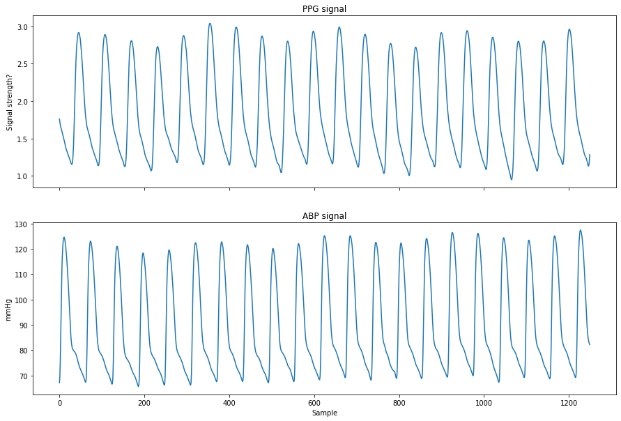
A comparison of the ABP and PPG signal is visible below: SBP and ABP comparison.

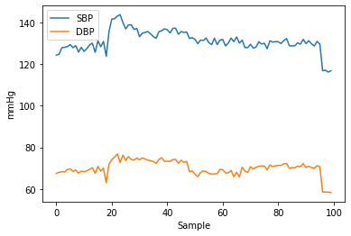
Inspecting the SBP and DBP shows they are good enough: SBP and DBP comparison.

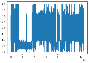
The PPG signal is surely non-ideal and that is why we will need to perform some further cleaning: PPG signal inspection.

For now we can create a baseline model and see how it fares. We did not extract any features yet so we do the prediction based only on the PPG signal:

# since we want to predict both SBP and DBP we will pack them for each sample
target_bp = []
for i in range(len(ppg)):
    target_bp.append((sbp[i], dbp[i]))

x_train, x_test, y_train, y_test = train_test_split(ppg, target_bp, test_size=0.3)

model = LinearRegression()
model.fit(x_train, y_train)
y_pred = model.predict(x_test)
mean_absolute_error(y_test, y_pred)

The achieved Mean Absolute Error was 13.8 which gives us some room for improvement. We need to extract features from the signal which may help us identify potential important characteristics for models.

Temporal and Spectral features extraction

Temporal

Since classic Machine Learning usually benefits from hand-picking some features from the input data, some features are extracted from the signal periods and assessed for validity. Features were chosen based on most popular ones in the recent scientific papers.

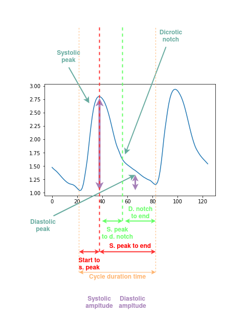
These include:

Cycle duration time
Time from cycle start to systolic peak
Time from systolic peak to cycle end
Time from systolic peak to dicrotic notch
Time from dicrotic notch to end
Ratio between systolic and diastolic amplitude

These features are explained in more detail in the graph underneath:

The code for extraction of both features is available in the [Jupyter notebook].

Spectral

Additionally, we can extract spectral features, which could help the models:

Three largest magnitudes (both values and frequencies)
Normalized energy
Entropy
Histogram - Binned distribution from 0 to 60 Hz (10 bins)
Skewness
Kurtosis

These features require some periodicity (remember our old friend Joseph Fourier?), so they have to be taken from ~10 periods of PPG.

Exploratory Data Analysis

After we obtained the features, we assemble the dataframes and clean them slightly.

rows = []

for i in range(len(ppg)):
    cycle_len, t_start_sys, t_sys_end, t_sys_dicr, t_dicr_end, ratio = extract_features_long_seg(ppg[i], ppg_ii[i])
    freq_1, mag_1, freq_2, mag_2, freq_3, mag_3, energy, entro, bins, skewness, kurt = extract_spectral_features(ppg[i])
    rows.append((cycle_len, t_start_sys, t_sys_end, t_sys_dicr, t_dicr_end, ratio,
                freq_1, mag_1, freq_2, mag_2, freq_3, mag_3, energy, entro, skewness, kurt, *bins))

rows = np.array(rows)

# make a df from the data to clean it
bins = [f"bin_{i}" for i in range(10)]
col = ["cycle_len", "t_start_sys", "t_sys_end", "t_sys_dicr", "t_dicr_end", "ratio",
       "freq_1", "mag_1", "freq_2", "mag_2", "freq_3", "mag_3", "energy", "entropy", "skewness", "kurtosis", *bins]
df = pd.DataFrame(rows, columns=col)

# drop rows with wrong values
idxs = df.loc[df['t_sys_end'] < 0.].index
inf_idxs = df.loc[df.values >= np.finfo(np.float64).max].index
indices = idxs.append(inf_idxs)
df = df.drop(indices)

# fill all NaN's
df.fillna(0, inplace=True)


# clean also the target variables
col = ["SBP" , "DBP"]
df_target = pd.DataFrame(target_bp, columns=col)
df_target= df_target.drop(indices)

Let’s take a quick look at the df.describe() which will tell us how the dataframe fares:

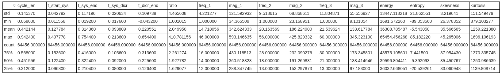
Briefly exploring the data, it can be seen there are some outliers which should be eliminated in order to make the models' predictions better. For this we will use IQR elimination - removing all the values which lie outside of the Q1 and Q3 percentile quarters in the normal distribution of the data:

# only some columns are striking, remove only rows where outliers are present in these columns
sus = ["ratio", "mag_1", "mag_2", "mag_3", "energy", "entropy", "skewness", "kurtosis"]
to_remove = set()

indices = set()
for x in sus:
  q25, q75 = np.percentile(df.loc[:,x], [25, 75])
  intra = q75 - q25

  max = q75 + intra * 1.5
  min = q25 - intra * 1.5

  idxs_1 = df.loc[df[x] < min, x].index
  idxs_2 = df.loc[df[x] > max, x].index
  to_remove = to_remove.union(idxs_1).union(idxs_2)

df.drop(to_remove, inplace=True)
df_target.drop(to_remove, inplace=True)

Now we can finally plot our data and see if there are any striking relations we should be aware of:

# correlation plots
plt.rcParams['figure.dpi'] = 100
plt.rcParams["figure.figsize"] = (20,15)
scatter_var = ["cycle_len", "t_start_sys", "t_sys_end", "t_sys_dicr", "t_dicr_end", "ratio",
               "freq_1", "mag_1", "freq_2", "mag_2", "freq_3", "mag_3", "energy", "entropy", "skewness", "kurtosis"]
correlation_matrix = df[scatter_var].corr()
sns.heatmap(correlation_matrix, annot=True)

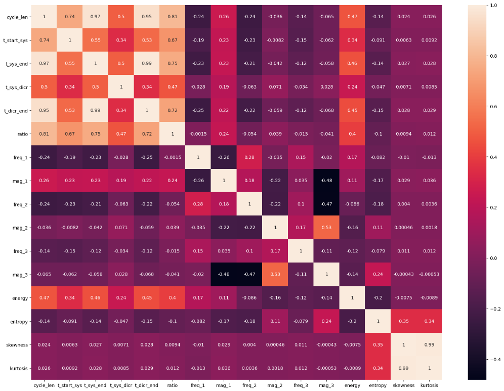
It can be seen that time features are quite correlated, which is expected. Also the energy is somewhat correlated with the time features. There are strong anticorrelations in frequency domain features - frequency/magnitude associations.

Apart from confirmation, this plot did not give as much insight as it can in other cases, so let’s move on!

Machine Learning and Results

Having the data prepared, we can now proceed with the training of various models to assess which one is the best. The most promising models in the literature are a Random Forest and Linear Regression so we are using them here as well. I won’t describe these two models here, because there is plenty of good sources on [RF] and [LR].

The data is further split using [K-Fold cross-validation], in order to train the model for a given number of epochs. Then it is finally used to predict on the intact test set.

folds = KFold(n_splits=10, shuffle=False)
# resplit the data after processing
x_train, x_test, y_train, y_test = train_test_split(df, df_target, test_size=0.3)

Finally, the model training can commence:

linear = LinearRegression()
errors_sbp = []
errors_dbp = []

for i, (train_idx, val_idx) in enumerate(folds.split(x_train, y_train)):
    train_data, train_target = x_train.iloc[train_idx], y_train.iloc[train_idx]
    val_data, val_target = x_train.iloc[val_idx], y_train.iloc[val_idx]

    linear.fit(train_data, train_target)
    predictions = linear.predict(val_data)
    error_sbp = mean_absolute_error(predictions[:,0], val_target["SBP"].values)
    error_dbp = mean_absolute_error(predictions[:,1], val_target["DBP"].values)

    print(f"Train fold {i} MAE SBP: {error_sbp} MAE DBP: {error_dbp}")
    errors_sbp.append(error_sbp)
    errors_dbp.append(error_dbp)

print(f"Average MAE SBP: {np.mean(errors_sbp)} MAE DBP: {np.mean(errors_dbp)}")

The results are visible in the picture below:

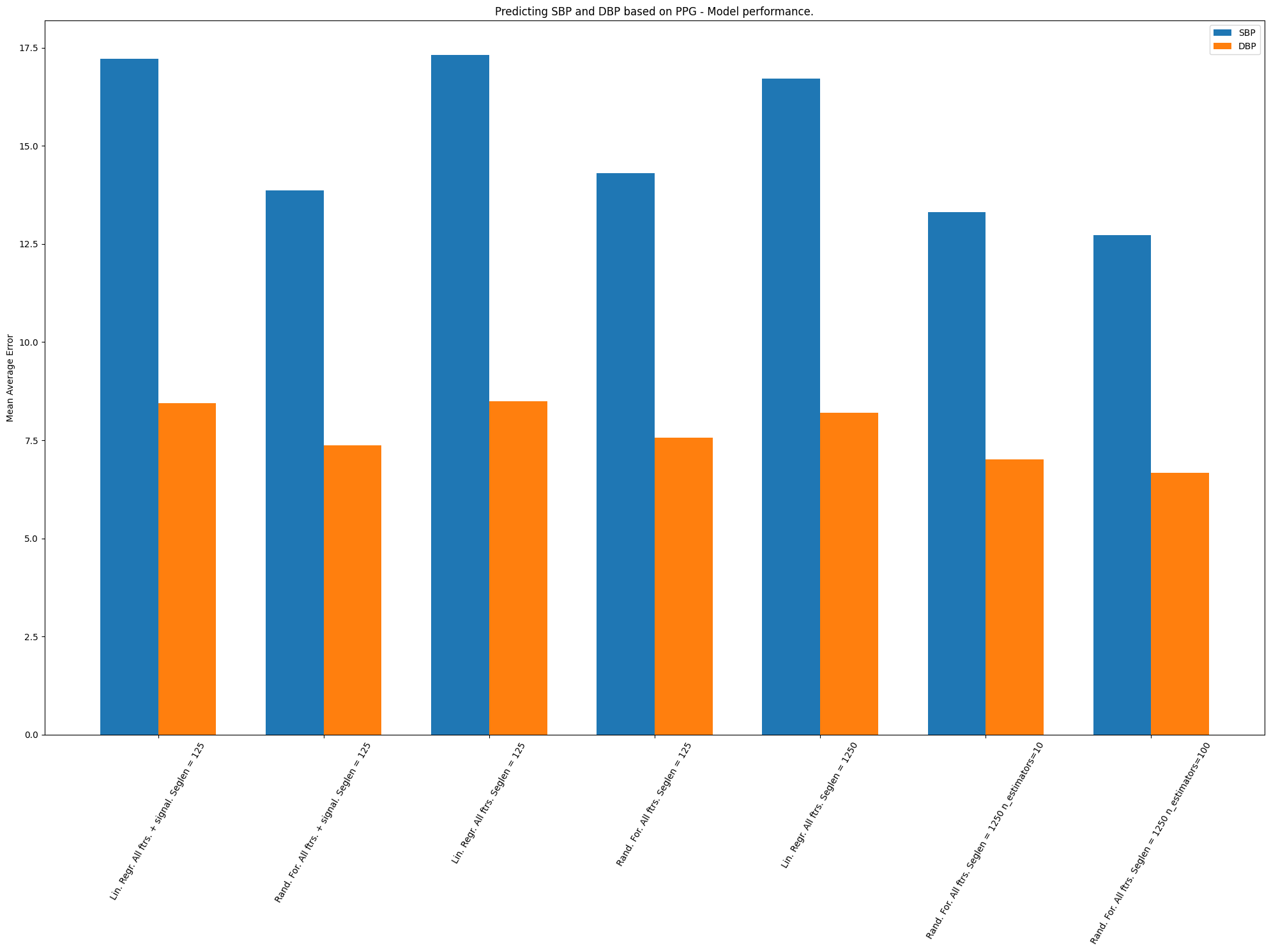
It is visible that the rightmost model is the most accurate - Random Forest with 10s segment lengths and 100 estimators. The results are far from ideal but they are not much worse than recent State of The Art (we have still much to improve in this area).

The most important problem we are now facing is making the data captured from the PPG with the Arduino fit our model (be normalized and rescaled). Also the PPG reading often wanders and has varying amplitude between readings, so we will have to rescale the data dynamically (averaging a period of 10 seconds or more).

Summary

This was the first of posts describing my endeavours with BIBoP, with several more to come. The next one will be focusing on AWS and setting up a Lambda which will make use of our model. I hope this post was informative enough and you learned something valuable.

As always, if you found anything unclear or want to provide feedback, reach out to me, be it below this post or personally 😄.

Also, if you like what I’m doing and you would like to see more of it - consider buying me a [coffee] ☕ [coffee]: https://www.buymeacoffee.com/jduchniewicz [Envidrawer]: https://www.element14.com/community/community/design-challenges/1-meter-of-pi/blog/2021/01/06/envidrawer-final-post [official repository]: https://github.com/JDuchniewicz/BIBoP [official contest website]: https://www.element14.com/community/community/design-challenges/design-for-a-cause-2021 [some]: https://www.element14.com/community/community/design-challenges/1-meter-of-pi/blog/2021/01/02/envidrawer-blog-7-ride-the-lightning [cool]: https://www.element14.com/community/community/design-challenges/1-meter-of-pi/blog/2021/01/03/envidrawer-4-3d-modelling-printing-and-further-assembly [concepts]: https://www.element14.com/community/community/design-challenges/1-meter-of-pi/blog/2020/11/02/envidrawer-2-materials-and-casing-assembly [Arduino Nano 33 IoT]: https://store.arduino.cc/arduino-nano-33-iot [cheatsheet]: https://gabriellesc.github.io/teaching/resources/GDB-cheat-sheet.pdf [like this one]: https://1bitsquared.de/products/black-magic-probe [Jupyter notebook]: https://github.com/JDuchniewicz/BloodPressurePPG [original post]: https://www.element14.com/community/community/design-challenges/design-for-a-cause-2021/blog/2021/05/13/bibop-3-blood-pressure-inference-machine-learning [UCI Machine Learning Repository]: https://archive.ics.uci.edu/ml/datasets/Cuff-Less+Blood+Pressure+Estimation [RF]: https://towardsai.net/p/machine-learning/why-choose-random-forest-and-not-decision-trees [LR]: https://www.cs.toronto.edu/~frossard/post/linear_regression/ [K-Fold cross-validation]: https://machinelearningmastery.com/k-fold-cross-validation/